Chertkov wiki — draft for Misha
The map an ENS listener from 9 April 2026 would want on the way home, if they decided to retrace the conceptual path from Schrödinger to bridge diffusions for ensembles of LLM agents.
Six-article map
| # | Article | One-line pitch |
|---|---|---|
| 1 | Schrödinger Bridge | The 1931 problem: reconcile a prior diffusion with two prescribed marginals at \(t=0\) and \(t=T\). |
| 2 | Path Integral Diffusion | Kappen's non-equilibrium framing — a bridge problem as an optimal control problem. |
| 3 | Harmonic Path Integral Diffusion | Behjoo & Chertkov — the anchor: an exactly solvable one-sample bridge under harmonic drift. |
| 4 | Mean-Field PID — samples that cooperate | Lift H-PID to \(N\)-sample ensembles with quadratic coupling; linear-interpolant theorem. |
| 5 | Compress-Add-Smooth — samples that remember | A second exactly solvable bridge; how a finite buffer carries information forward. |
| 6 | Decision Flow | Discrete outlook on the same bridge hierarchy. |
flowchart TD
    SB["(1) Schrödinger Bridge"] --> PID["(2) Path Integral Diffusion"]
    PID --> HPID["(3) Harmonic PID<br/>(anchor — already landed)"]
    HPID --> MF["(4) MF-PID<br/>samples that cooperate"]
    HPID --> CAS["(5) Compress-Add-Smooth<br/>samples that remember"]
    HPID --> DF["(6) Decision Flow<br/>discrete outlook"]
A figure I would like to show you
Below is a single observable on one slice of data from five independent multi-agent LLM systems running real coding and writing tasks (2026-04-11 to 2026-04-20, N=272 sessions, all caveats stated below). It is not a distributional bridge ensemble — the observable (\(x(t) = \mathrm{cum\_events}/\mathrm{total\_events}\)) is monotone and pinned by construction; in that sense the trace of any monotone counter that ran from start to finish would look the same shape. The thing my eye keeps going back to is the fanning between the endpoints, and the way the per-fate medians separate before \(t \approx 0.05\). Whether that fanning is dynamical information or bookkeeping noise is the first thing I do not know how to read.
The figure sits here as one possible entry point. The six articles above are the preparation I did to have the vocabulary for the conversation ; they are not a thesis.
A few of the questions I have been turning over. What does it mean that the endpoints are pinned by construction and not by dynamics? Is the right move to enrich the model around this observable, or to change the observable while keeping the data? Several of your bridges (MF-PID, GH-PID, AdaPID, Compress-Add-Smooth, Decision Flow) might each read this object differently — I have not picked one, and I would rather hear which one you reach for than guess. Honest possibility: the right reading is none of the above, change the observable — for instance to responsibility entropy over persona outputs, or an embedding-space position of the work artefact.
This is data I have, not a claim I am making. The shape is suggestive; the right reading is the part I do not yet know how to do.
Part 1 — the picture, in plain words
I recorded 272 conversations in which a large-language-model assistant worked on real coding and writing tasks. Each conversation starts with a task being posed, advances by small logged steps, and ends when the assistant either finishes, is stopped by a human, or gives up. I took all 272 conversations, rescaled each one so that \(0\) is its first heartbeat and \(1\) is its last, and stacked them on a single plot. Each thin line is one conversation; each colour is what kind of ending it had.
Part 2 — what was measured, and how
Source. Append-only event logs
(events.jsonl) written by five independent Python and Rust
software-engineering projects, each running its own internal task
scheduler for LLM-assistant work. Period: 2026-04-11 to 2026-04-20. No
synthetic bootstrapping — only events that were actually logged during
real work sessions.
Selection. An agent trajectory is kept only if it has at least three logged events and at least 30 s of wall-clock life. Shorter traces are instrumentation artefacts: aborted starts, re-runs, and heartbeat-only records. This filter discards false-starts and pure bookkeeping noise.
Time rescaling. For each trajectory \(m\) with first event at wall-time \(\tau_0\) and total wall-duration \(T_m\), rescale
\[ t \;:=\; (\tau - \tau_0)\,/\,T_m \;\in\; [0,1]. \]
The initial and terminal edges are pinned by construction: every trajectory has a recorded first event (\(t=0\)) and a recorded last event (\(t=1\)).
Observable.
\[ x(t) \;=\; \mathrm{cum\_events}(t)\,/\,\mathrm{total\_events} \]
— a monotone non-decreasing step function per trajectory, read as cumulative progress.
Terminal fate. Three classes, labelled from the first terminal event: finished successfully (the trajectory reached a completion event); interrupted (a human guardrail stopped it before completion); self-abandoned (the worker itself declared failure and exited). Counts: \(228 / 44 / 0\) respectively. Zero trajectories in the self-abandoned class — a bookkeeping detail about the period observed, not a claim of quality.
Reading. Per-fate median trajectories (thick lines)
separate early; the dashed marker at \(t^\star\) is the earliest grid point where
the inter-fate median spread exceeds one inter-fate \(\sigma\). Uniform reference \(x(t)=t\) shown for calibration. The figure
is fully reproducible via
experiments/speciation-v0/run.sh.
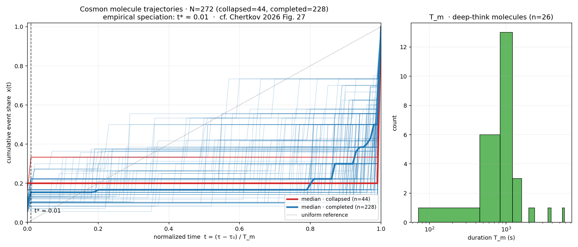
Caveats (stated, not hidden). (i) Finite \(N\): 272 trajectories across five projects, secretariat-dominated (220 / 272). (ii) Bookkeeping signature near \(t \approx 0.01\): one instrumental event fires within \(\sim 10\) ms of every first event, so the very-early per-fate spread is instrumentation, not a biological bifurcation. (iii) Fate labels use the first terminal event only; late status changes are ignored. (iv) No cross-project clock-drift correction.
What the figure does not do. It does not test MF-PID. It shows that the raw data is there, at scale, in a form compatible with the bridge reading — pinned endpoints, rescaled time, a monotone observable per trajectory, a clean fate partition — and it invites the next step: to co-construct a falsifiable observable on this data, aligned with slides 27 and 46 of the ENS talk (speciation transition, responsibility entropy).
Where the conversation could go
Three questions, in roughly the order they came to mind. Any one of them is a good Thursday conversation; none of them is the question I am sure of, and a "none of the above, look at this instead" answer is equally welcome.
On the figure — is it the right object? The plot is monotone counters pinned at the endpoints — a clock with a label more than a trajectory in any deeper sense. If you were handed the raw event stream, the per-session metadata, the fate label — what observable would you compute first? Responsibility entropy over per-step outputs, an embedding-space position of the work artefact, a KL distance against a Brownian-bridge reference — or something I have not considered?
On the cooperate / remember dyad. MF-PID names samples that cooperate via quadratic mean-field coupling; Compress-Add-Smooth names samples that remember via finite-buffer capacity (\(a_{1/2} \approx c \cdot L\)). For an ensemble where agents share a buffer of past sessions and a workflow scheduler — are these two mechanisms compositional, or does one preclude the other?
On the discrete outlook. Decision Flow is the discrete counterpart of the diffusion-time bridges. Multi-agent workflows are discrete-state, discrete-time graphs with a prior transition kernel (the scheduler) and an empirical terminal distribution (the fate labels). For a reader trying to choose between a discrete and a continuous reading of an agent ensemble — what diagnostic tells you the discreteness is load-bearing?
Corrections and sharper framings on any of the six articles are actively welcome.
Primary sources
- Schrödinger, Über die Umkehrung der Naturgesetze, Sitzungsber. Preuß. Akad. Wiss., Phys.-Math. Kl. (1931), 144–153. English translation with commentary: Chetrite, Muratore-Ginanneschi, Schwieger, arXiv:2105.12617 (2021).
- Léonard, A survey of the Schrödinger problem and some of its connections with optimal transport, arXiv:1308.0215 (2014).
- Chen, Georgiou, Pavon, On the relation between optimal transport and Schrödinger bridges, J. Optim. Theory Appl. (2016).
- Kappen, Path integrals and symmetry breaking for optimal control theory, J. Stat. Mech. (2005).
- Chernyak, Chertkov, Bierkens, Kappen, Stochastic optimal control as non-equilibrium statistical mechanics, DOI:10.1088/1751-8113/47/2/022001 (2014).
- Behjoo, Chertkov, Harmonic Path Integral Diffusion, arXiv:2409.15166 — IEEE Access DOI:10.1109/ACCESS.2025.3548396 (2025).
- Chertkov et al., Mean-Field PID — GH-PID, arXiv:2512.11859 (2025).
- Chertkov et al., AdaPID, arXiv:2512.11858 (2025).
- Chertkov, Compress-Add-Smooth (sole-authored), arXiv:2604.00067 (2026).
- Chertkov, Ahn, Behjoo, Decision Flow, arXiv:2503.14549 (2025).
Draft, 2026-04-20 — Emmanuel Sérié. Built with the assistance of an agent-orchestration system in development. Corrections welcome.